Connections¶

Total stations and digital levels usually support a serial connection with RS232. Some instruments come with additional connection methods, like bluetooth as well.

Serial Line¶

The RS232 serial line is the main method of connection. The relevant main primitive is the SerialConnection class, that acts as a wrapper around a Serial object that implements the actual low level serial communication.

1
2
3
4
5
6
7
8

from serial import Serial
from geocompy.communication import SerialConnection


port = Serial("COM1", timeout=15)
com = SerialConnection(port)
com.send("some message")
com.close()  # Closes the wrapped serial port

The SerialConnection can also be used as a context manager, that automatically closes the serial port when the context is left.

1
2
3
4
5
6
7

from serial import Serial
from geocompy.communication import SerialConnection


port = Serial("COM1", timeout=15)
with SerialConnection(port) as com:
    com.send("some message")

To make the connection creation simpler, a utility function is also included that can be used similarly to the open() function of the standard library.

1
2
3
4
5

from geocompy.communication import open_serial


with open_serial("COM1", timeout=15) as com:
    com.send("some message")

If a time consuming request has to be executed (that might exceed the normal connection timeout), it is possible to run it with a temporary override.

 1
 2
 3
 4
 5
 6
 7
 8
 9
10
11
12

from geocompy.communication import open_serial


with open_serial("COM1", timeout=5) as com:
    ans = com.exchage("message")
    # normal operation

    # request that might time out
    with com.timeout_override(20):
        ans = com.exchange("blocking message")

    # resumed normal operation

Bluetooth¶

Newer instruments (particularly robotic total stations) might come with built-in or attachable bluetooth connection capabilities (e.g. Leica TS15 with radio handle). These instruments communicate over Serial Port Profile Bluetooth Classic (SPP), that emulates a direct line serial connection.

To initiate a connection like this, the instrument first has to be paired to the controlling computer, and the bluetooth address of the instrument must be bound to an RFCOMM port as well.

Windows¶

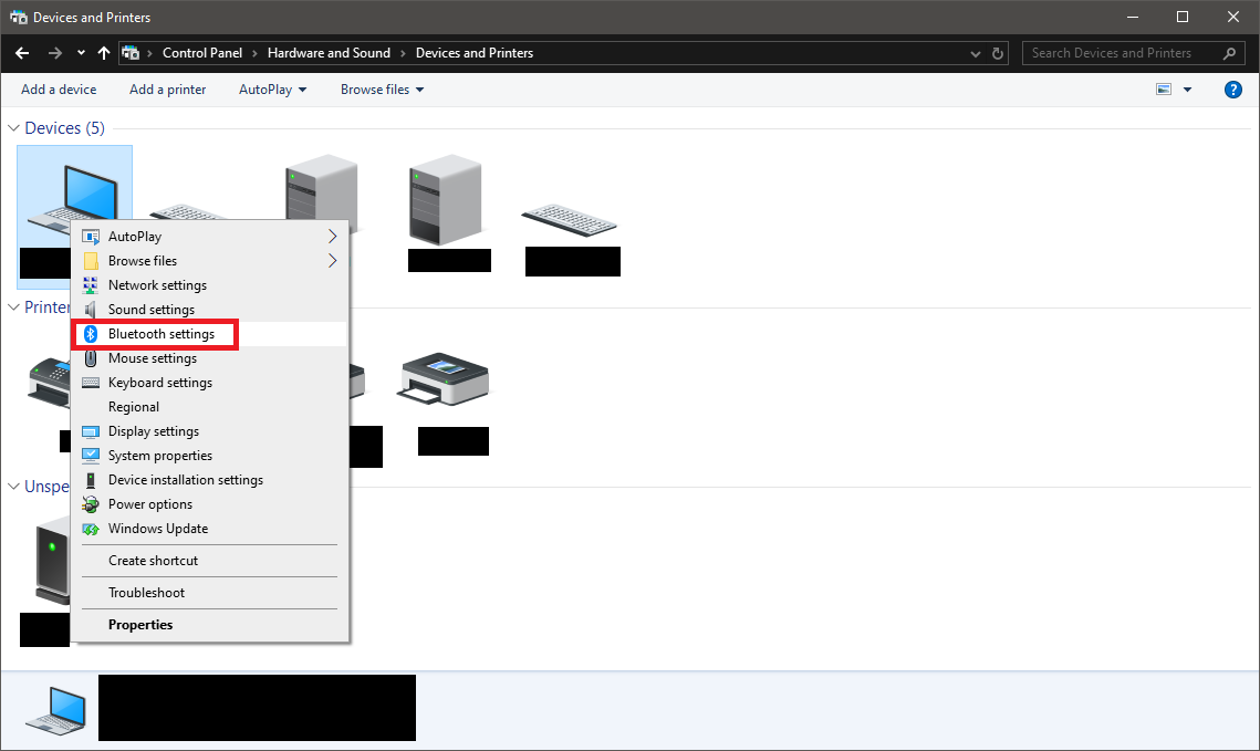
On windows machines the process is relatively straight forward. New SPP devices can be added through the “Devices and Printers” page of the Control Panel.

1. Right-click on local computer and select the Bluetooth settings

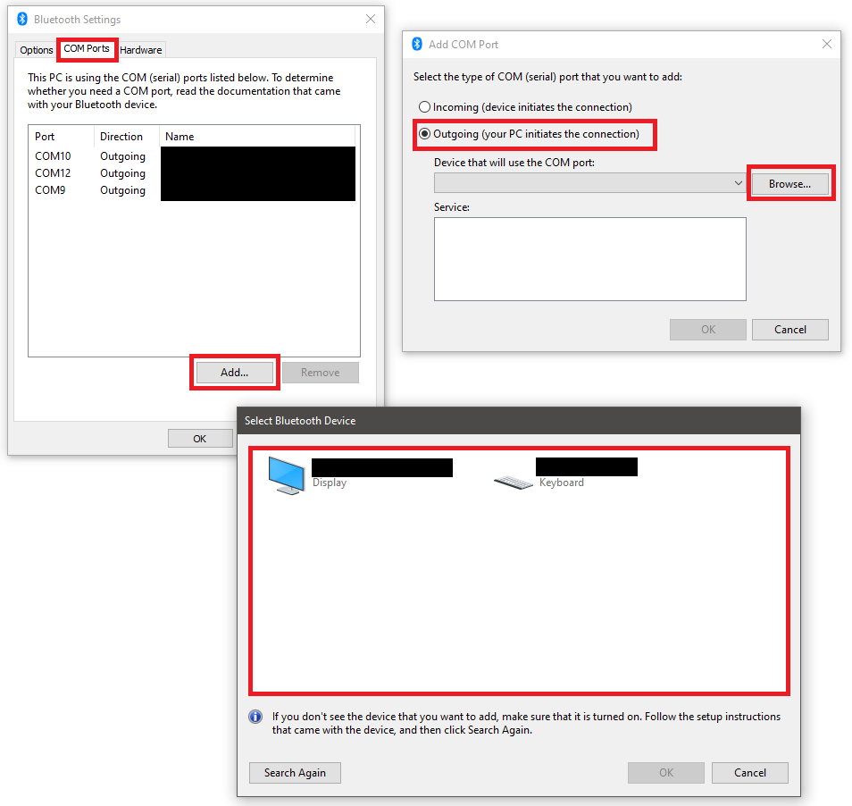
2. Navigate to the COM Ports tab

3. Click on Add

4. Select the Outgoing connection option and click Browse

5. Wait for the device to show up in the discovery window, then press OK

6. Click OK in all the windows

If the process is successful, a new device will be added to the list of devices. To double check, that the COM port binding was successful, open the properties of the new device, and check, that the SPP service is active and what port was assigned to it.

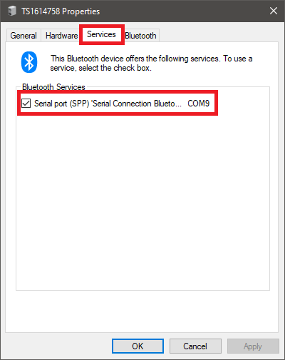
The actual device pairing will be initiated when the first actual connection is attempted. The pairing code is usually 0000 or 1234.

Linux¶

To add an SPP Bluetooth connection, the Bluetooth service has to be set to compatibility mode, and the SPP service registered. This can be done by updating the config of the bluez service.

sudo nano /etc/systemd/system/dbus-org.bluez.service

Two lines have to be modified/added in the config:

ExecStart=/usr/lib/bluetooth/bluetoothd -C
ExecStartPost=/usr/bin/sdptool add SP

After the modifications the Bluetooth service has to be restarted (the cleanest solution is to simply restart the whole Raspberry Pi).

Once restarted, check, that the service started without issues:

service bluetooth status

If the service started without errors, the pairing and binding can be done.

Start the Bluetooth utility:

bluetoothctl

Make sure, that the device modem is powered on, the agent is active and start scanning:

power on
agent on
scan on

Wait for the device to appear (Bluetooth MAC address and device name), then turn off the scanning:

scan off

Once the MAC address is known, the device can be paired and set to trusted (the pairing code is usually 0000 or 1234):

pair <MAC address>
0000
trust <MAC address>

After the pairing is successful, the devices can be checked:

paired-devices

If everything is done, the utility can be closed:

quit

The final step is creating the RFCOMM binding, that allows to access the SPP service connection:

sudo rfcomm bind hci0 <MAC address>

The existing RFCOMM bindings can be checked if needed:

rfcomm

If the whole process was successful, the device will be accessible on the /dev/rfcomm0 port, and can be used as any direct line serial connection.

1
2
3
4
5

from geocompy import open_serial


with open_serial("/dev/rfcomm0") as com:
    com.send("some message")

Internet¶

The newest instruments (in addition to Bluetooth) also come with WLAN support. This enables connections through TCP/IP.

To initiate a connection through internet sockets, the instrument and the controlling computer must be connected to the same WLAN.

1
2
3
4
5

from geocompy import open_socket


with open_socket("192.168.0.1", 1212, "tcp") as soc:
    soc.send("some message")

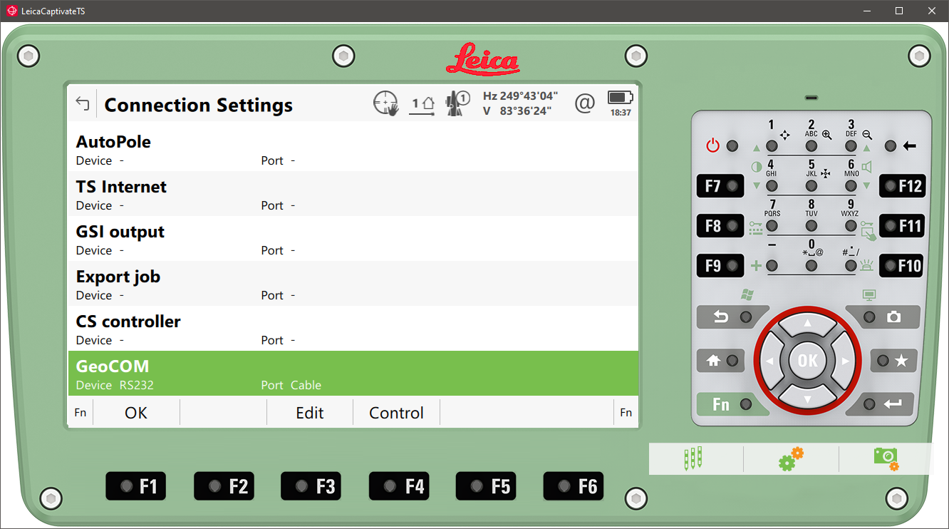
Simulators¶

For testing and development purposes it is possible to make a connection to the Leica Captivate TS simulator (and possibly other older official instrument simulators). The simulators are available with an existing Captivate license, or individual request from Leica or a Leica dealer.

To communicate with the simulator, a virtual serial port pair needs to be set up on the computer. An open source solution is to use com0com.

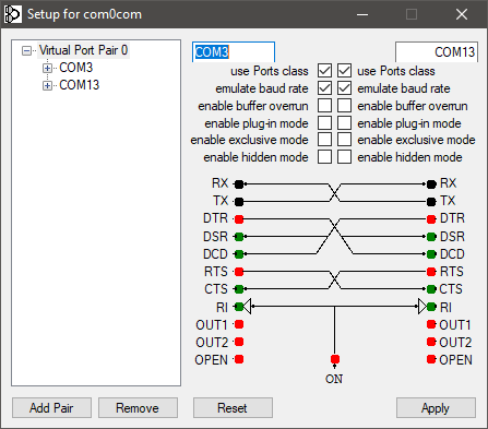
It installs virtual serial port emulator drivers to simulate connections. The communication is channeled through the presistent virtual devices.

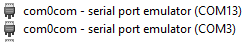
In the settings of the simulator, the cable connection can be set to one end of the virtual port pair (COM3 in this example), the other end can be used to connect to the simulator (COM13 here).

The interface settings have to be set accordingly in the simulator itself, just like on a real instrument.

Realiability¶

Some connections might not be as reliable as needed for stable operation. Interference can cause messages to get corrupted, or not arrive at all at the destination. For stable operation there must be a way to detect a missing or corrupt message.

The GeoCOM protocol supports two mechanisms to detect faults in communication. The GSI Online system has no such support.

Transactions¶

The GeoCOM request and response messages can optionally have a transaction ID field.

%R1Q,0:
%R1P,0,0:0

%R1Q,0,1:
%R1P,0,1:0

When the ID is incremented for each request-response exchange, it can be used to detect if the two ques get misaligned due to a missing response. This can happen if the connection times out, but the instrument still sends a reply after the timeout period. This would leave an unread message in the receiver buffer, which would get confused with the response to the next request.

%R1Q,0,3:
%R1P,0,2:0

Transaction IDs must be in the positive range of a 16 bit signed integer (0 - 32767). After 32767, the ID must roll back to 0 (otherwise the instrument will respond with overflowed IDs -32768, -32767, etc.).

Checksums¶

While transactions can be used to detect out of sync request-response ques, they cannot detect partially corrupted messages (a corruption that leaves the message syntactically correct, but with altered meaning).

To detect corrupted messages, GeoCOM requests and responses have an optional checksum field. The checksum is calculated with the CRC-16/ARC method.

When sending a request, the checksum has to be first calculated for the message without the checksum field, then the checksum must be inserted before the message is sent.

with open_serial("COM1") as com:
    cmd = "%R1Q,0,11:"
    checksum = crc16(cmd)
    cmd = f"%R1Q,0,11,{checksum}:"
    com.send(cmd)

After receiving the response, the checksum must be first extracted from the message, then recomputed from the response without the checksum. If the received checksum and the computed checksum are equal, the message is intact. Otherwise an error occured during transmission.

with open_serial("COM1") as com:
    resp = com.receive() # example: resp = "%R1P,0,11,22896:0"
    parts = resp.split(":")
    header = parts[0].split(",")
    checksum_rec = int(header[3])
    checksum_calc = crc16(",".join(header[:3]) + ":" + parts[1])
    if checksum_rec != checksum_calc:
        raise ValueError("Checksum mismatch")

with open_serial("COM1") as com:
    tps = GeoCom(com, checksum=True)